
Plotting
Polar Plots are available through a distinct window launched from the Plot menu on the QSAS main window as a separate 2D Polar Plot menu item.
The 2D Polar Plot window has three tabs, Data, Plot Options and Page and plots into its own
plot window which is independent of the main plot window. In addition to the usual Plot button, this
plot viewer also provides an Animate Time button which will successively plot each data record in the input data object
from the current time slider position to the end. Animate Time will first calculate a suitable colourscale for the whole time interval
if the Auto Colourscale toggle is on, and this may cause a delay before animation starts with large data sets.Animations may be slowed down with the Animation Delay control.
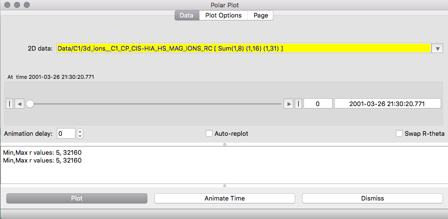
The Data tab has a data drop slot which expects a 2 dimensional array or array sequence. If a higher dimensional data object is dropped in it will use the default array reduction set in the user's profile in order to sub-sample down to 2 dimensions. This selection can be modified using the slot pulldown. When a time series object is dropped in, the record/time slider is active and the record to be plotted can be selected with the slider or typed into its record field. If the Auto-replot button is selected, then changing the record will automatically replot the data at the new record. The plot will automatically choose the first dimension with units of degrees or radians as the angular dimension, but this can be over-ridden using the Swap R-theta button.
The Plot Options tab allows the user to control the plot design, but defaults for all options are set according to the data and its metadata. The plot and axis titles can be explicitly set in the appropriate fields. The Plot can either be Arc-Filled (solid blocks of colour for each bin bounded by the DELTA_PLUS and DELTA_MINUS metadata of the DEPEND_1 and DEPEND_2 attributes) or Shaded (smooth colour shading between neighbouring data points). The X and Y axes are always plotted, and in addition either an extra radial axis scale or bounding box can be set with the Axis Type field. The weight and length of the axes can be set using Axis width and Axis extent to allow extra white space around the plot for clarity of labelling.
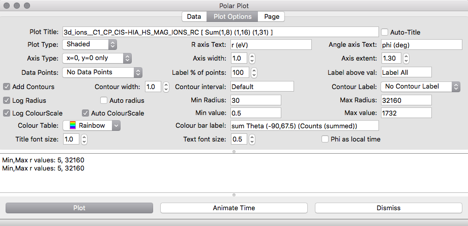
The positions of the actual data points (which may NOT be bin centred in the DELTA_PLUS and DELTA_MINUS are different) can be plotted on top, and these may be labelled with the actual data value. Since labeling data points can make for over-full plots, the percentage of data points labelled can be set independently, and it is also possible to limit data labeling to be those above a certain value set in Label above val field.
The Add Contours toggle will allow contours to be overplotted, and the contour interval and contour labelling can be controlled. When a logarithmic colour scale is chosen the contour interval will refer to the interval in the power of 10.
The Radial dimension can be plotted in the log, in which case zero or negative radial values are automatically excluded. If the radial quantity is anywhere negative then, when log radius is selected, the minimum value in r is subtracted from each radial value and this offset noted in the text pane. In addition the first non-zero radial value is used as lower limit, but this may be over-ridden by manually setting the radial minimum value. Negative radial values are permitted for linear radial plots. In all cases the centre of the circle need not be at zero radius, and selecting a minimum value below the lower data limit may result in a hole in the centre of the plot when the plot type is Shaded, whereas Arcfill plots always fill the last bin down to the origin.
Similarly the z dimension (colourscale) may be logarithmic, in which case the lowest non-zero value is used when autoscaling.
The colour scale range may be manually over-ridden.
The font sizes for title and text can be controlled independently,
and the Phi angle can be represented as local time rather than degrees
(midnight is at zero degrees).
The Page tab controls the paper size, resolution when printed (where appropriate) and paper orientation. Custom paper sizes can be specified, and all measurements are in the units set in the Units field.
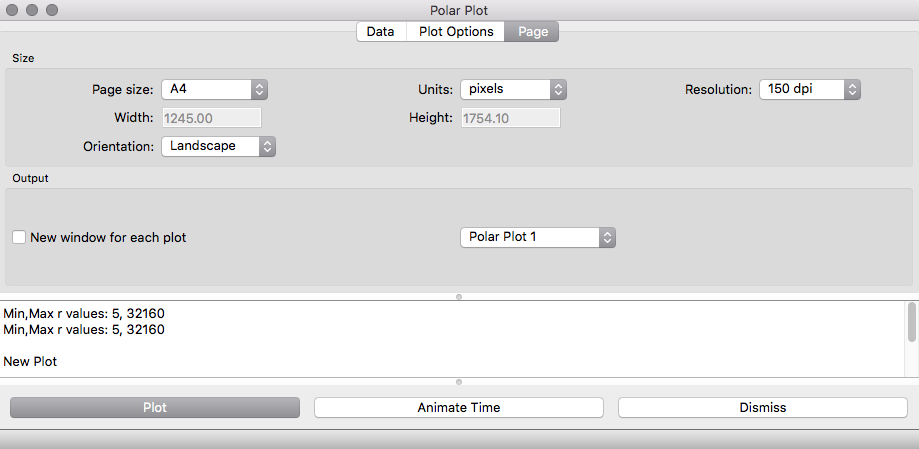
Under normal use each plot will appear in the same window created the first time Plot is pressed. The New window for each plot toggle allows a fresh window to be created each time Plot is pressed, and selecting the Plot window id of an existing window allows it to be overwritten (after deselecting New window for each plot).
Printing or saving a plot to a file is achieved using the Plot menu from the plot pane itself after plotting.
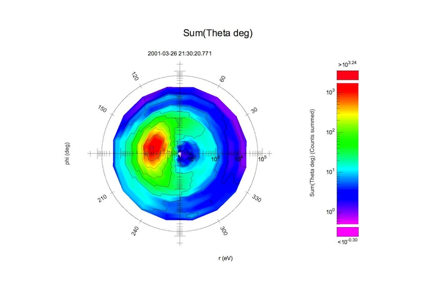
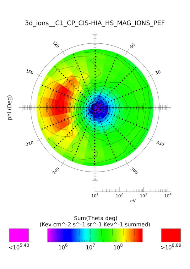
The Sample session shipped with QSAS contains a saveset
(Sample_Ions.qx_polar_plot) for a 2D polar plot of the ion data in the
sample session.
The resulting plot should look as follows:
Using the portrait page orientation with Arcfill and show data point selected and different range options this plot becomes:
Last up-dated: October 2016 Tony Allen