
Plotting
Polar and Cartesian 3D data views are available through a
distinct window launched from the Plot menu on the QSAS main
window as a separate 3D View menu item.
The 3D View window has three tabs, Data, Plot Options and Page and plots into its own plot window which is independent of the main plot window.
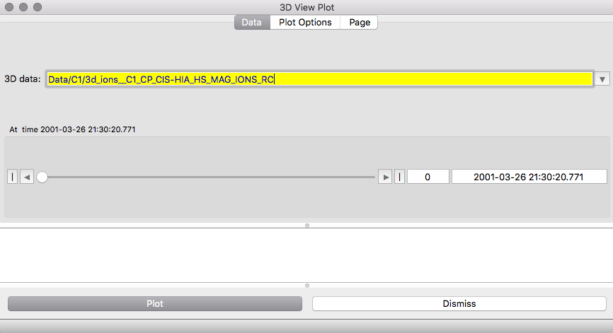
The Data tab has a data drop slot which expects a 3 dimensional array or array sequence. When a time series object is dropped in, the record/time slider is active and the record to be plotted can be selected with the slider or typed into its record field. If the Auto-replot button is selected, then changing the record will automatically replot the data at the new record. The plot will automatically choose the first two dimensions with units of degrees or radians as the angular dimension in polar plots, but this can be over-ridden using the R dimension selector on the options tab.
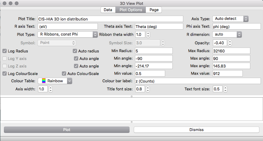
The Radial dimension (and all cartesian dimensions) can be plotted in the log, in which case zero or negative values are automatically excluded. If the radial quantity is anywhere negative then, when log radius is selected, the minimum value in r is subtracted from each radial value and this offset noted in the text pane. In addition the first non-zero radial value is used as lower limit, but this may be over-ridden by manually setting the radial minimum value. Negative radial values are permitted for linear radial plots.
Similarly the data dimension (colourscale) may be logarithmic,
in which case the lowest non-zero value is used when autoscaling.
The colour scale range may be manually over-ridden.
The font sizes and line width for axes can be controlled.
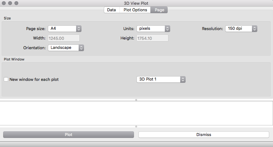
The Page tab controls the paper size, resolution when printed (where appropriate) and paper orientation. Custom paper sizes can be specified, and all measurements are in the units set in the Units field. Page controls are the same as for the 2D polar plots.
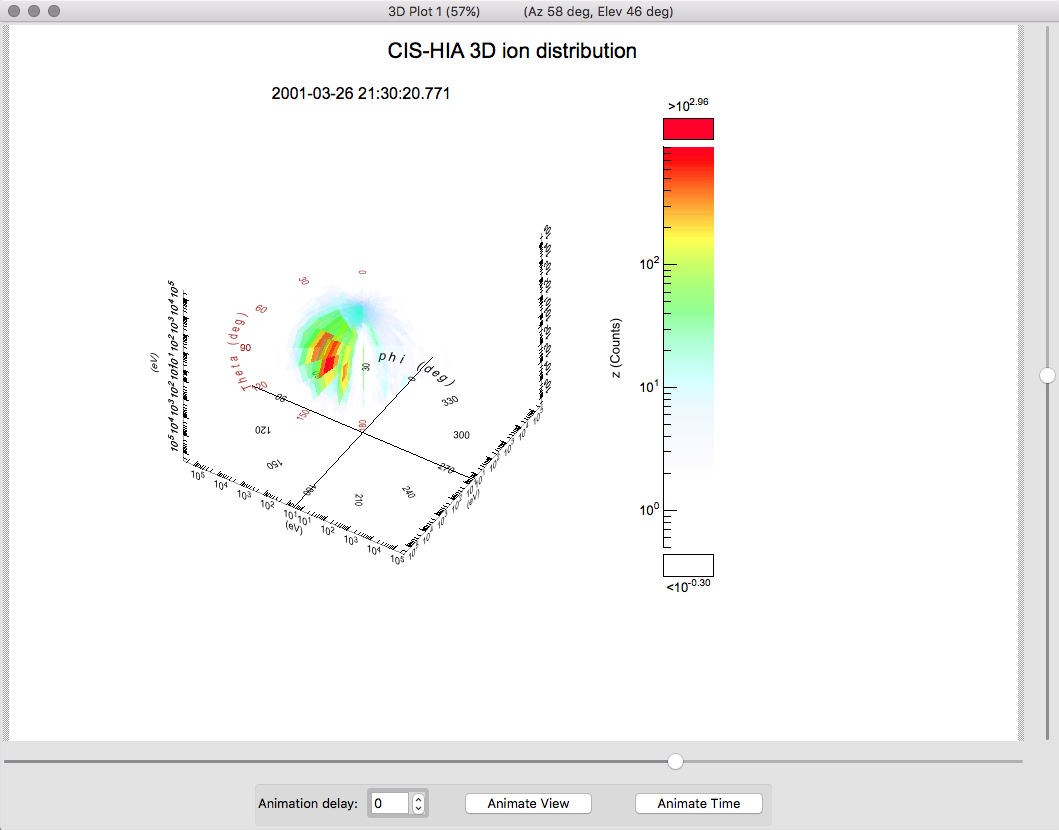
The viewing angle for the plot can be
controlled by the sliders on the 3D plot pane, and the viewing
angle is shown on its title bar.
The 3D plot pane itself holds an Animate View
button which will continually change the viewing angle for 30
seconds, starting from the current viewing angle, and an Animate
Time button which will successively plot each data record in the
input data object from the current time slider position to the
end. Animate Time will first calculate a suitable colourscale
for the whole time interval if the Auto Colourscale toggle is
on, and this will cause a delay before animation starts with
large data sets.
Under normal use each plot will appear in the same window created the first time Plot is pressed. The New window for each plot toggle allows a fresh window to be created each time Plot is pressed, and selecting the Plot window id of an existing window allows it to be overwritten (after deselecting New window for each plot).
Printing or saving a plot to a file is
achieved using the Plot menu from the 3D plot pane itself after
plotting.
The Sample session shipped with QSAS contains a saveset (saveSet.qx_3dview_plot) for a 3D ribbon plot of the ion data in the sample session with the opacity set to -0.4 to emphasise the location of the data peak. The resulting plot should look as follows:
Last up-dated: October 2016 Tony Allen